How To Draw Linear Programming Graph In Excel

Problem

Y'all've formulated an optimization problem in traditional linear programming course and would similar to use Excel to solve the problem.

Solution

Use Solver'due south linear optimization capabilities.

Discussion

Linear optimization issues can be written in the form of an objective function to maximize (or minimize) subject field to constraints. Constraints can be written in the form of inequalities or equalities. Consider this simple instance:

Objective function

Constraints

If this were a product mix blazon of trouble, the variables x1 and x2 could correspond different products subject to some availability or production constraints, while the objective function could correspond total profit given the mix of products produced. The thought is to notice the optimum mix of products so as to maximize profit. Linear optimization is not limited to this sort of product mix trouble. For example, your problem could consist of trying to maximize the vitamin content of a livestock feed given certain ingredients, subject to their availability and cost. Or your problem could consist of trying to minimize the cost of labor for producing certain products in your laboratory (meet the adjacent recipe for a hypothetical example).

Moreover, the problem need not be limited to two variables. You tin can accept any number of variables and constraints, depending on your problem. I chose 2 variables for this simple example because we tin plot it using Excel's charting feature and gain some insight into the solution. Issues with more variables are much more difficult, if not impossible, to visualize adequately. Such problems require you lot to exercise great intendance when searching for a solution (peculiarly if the trouble is nonlinear) or to simplify the trouble in ways that volition allow you to visualize certain variables while holding others constant.

Getting back to our simple example, Effigy 13-ane shows a graph of our problem. I used Excel'southward charting features (see Affiliate 4) to prepare this graph.

This graph essentially consists of the constraints for the trouble within the x1, x2 space. The ii direct lines labeled Constraint 1 and Constraint 2 correspond the first two constraints. The shaded region beneath these constraints represents the region of viable values for x1 and x2 that are within the given constraints. Notice that this region is bounded by the x1- and x2-axes because we also have the two greater-than-or-equal-to-null constraints on these variables.

Figure 13-one. Graph of linear optimization example

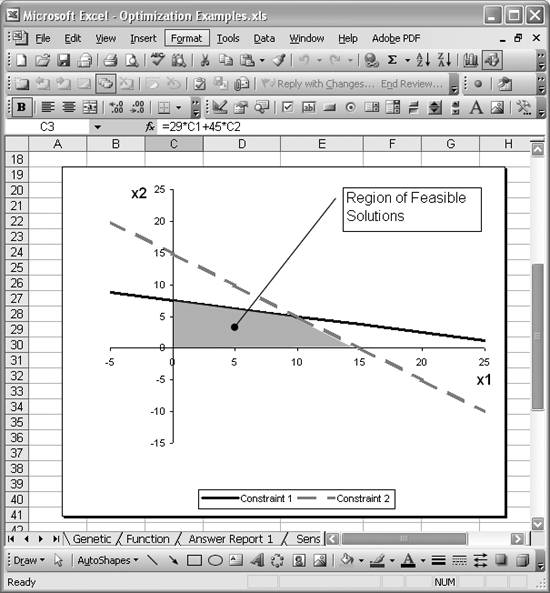
From this graph, you can deduce that the optimum solution corresponds to (x1,x2) = (10,5), which is at the intersection of the two constraint lines. You lot can use Solver to verify this result.

Effigy 13-2 shows a simple spreadsheet I gear up to facilitate finding optimum values for x1 and x2 and so every bit to maximize the objective function.

Figure thirteen-2. Linear optimization case

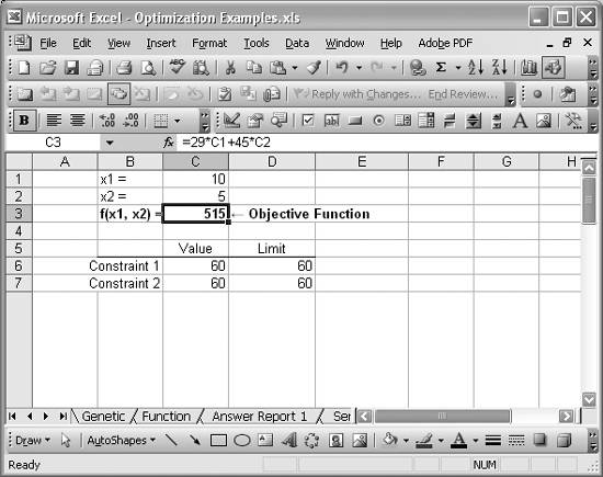
Cell C3 contains the righthand side of the objective office. The formula is =29*C1+45*C2. The values for x1 and x2 shown in Figure 13-2 are indeed the optimum values, and the value of 515 for the objective function is the maximum value. Earlier calling Solver, cells C1 and C2 contain only initial guesses for the optimum. I had initially prepare these to 0.

Cells C6 and C7 contain formulas corresponding to Constraint ane and Constraint two, respectively. The formula in C6 is =2*C1+8*C2, and the formula in C7 is =4*C1+4*C2. These formulas represent the lefthand side of the constraint equations shown earlier. The limiting values (called righthand side values) for these constraints are independent in cells D6 and D7.

Effigy 13-iii shows the Solver model I used to solve this problem.

The target cell is C3 and I instructed Solver to attempt to maximize its value. The cells to change are C1 and C2, respective to x1 and x2, respectively. There are four constraints besides. Refer to Recipe 9.4 to learn how to add constraints in Solver.

Figure 13-3. Solver model for linear optimization

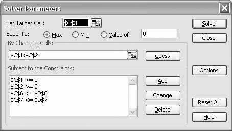
The first two constraints shown in Figure 13-3 represent to the constraints that x1 and x2 must exist greater than or equal to 0. The final two constraints correspond to the constraint equations discussed earlier, that is, Constraint 1 and Constraint 2 as plotted in Figure thirteen-1.

I also set the Solver option Presume Linear Model for this problem, since it is a linear optimization problem. See the introduction to Chapter ix for a give-and-take of Solver's options. Pressing the Solve button results in the optimum solution shown earlier in Figure 13-2.